You will need
- Table editor Excel 2007
Instruction
1
If you want single action - multiply two numbers – the sequence of actions should be:
- click in the blank cell, Excel spreadsheet (by using the navigation arrow keys and by clicking the desired cell with the mouse);
- press the "=". Excel interpreterpath this action as the beginning of the input formula;
- now print the desired mathematical operation using as a multiplication sign, the asterisk (*). Signs of mathematical operations called "operators". For example, if you multiply 2 by 3, then the cell you need to type "=2*3, where the equal sign is left from the previous step, re-print it is not necessary. If you want to multiply, not two, but more numbers - nothing changes in the rules print more. For example, =2*3*4*7*12;
- when you enter press Enter. Excel will calculate the result and show it in the same cell.
Instead of the usual write math using the multiplication operator (*), you can use the function with name PRODUCED. In this case, the content of a table cell, carrying out the multiplication of the five numbers will look like this: =K(2;3;4;7;12).
2
If it is necessary to organize a permanent form of multiple cells to one of them to print the multiplicand in the other the multiplier, and the third to see the result of the multiplication:
- in the first empty cell type the number (multiplicand) and press Enter;
in the second empty cell, type the second number (multiplier) and press Enter;
in the third cell, press "=" and using the navigation keys (arrows) move to the first cell (containing multiplicand). Alternatively, you can just click the cell with the mouse. Having done this, press the asterisk (multiplication operator). The cursor will return to the third cell, but you need by using the same navigation keys or mouse to move to the second cell containing the multiplier. After that, the contents of the cell with the formula should look like this: =A1*A2. Having done all that, hit Enter to finish entering the formula in the third cell you will see the result of the multiplication.
You have built a mini-calculator - now you can change the number mnogiego and multiplier, and Excel in the third cell to display their work.
And here multiply numbers does not necessarily have to be only two acting exactly the same way you can organize the desired number of multiplies of cells with numbers. But in this case it is more convenient to use the operator * and the function. Then you won't have to specify each cell number individually, you can specify a range of cells. For example, if you put multiplies the numbers in cells starting with A1 and ending with the A8, then the contents of the cell showing the result of multiplying them all should be: =K(A1:A8). The cell range can be entered in the function "manually", and you can select with the mouse and Excel will enter the desired value itself.
3
If you need a single multiply the value of each cell in the column (or row) of the table on some index:
- in any blank cell, type this number is the coefficient;
- then select that cell, on the Home tab, in the very first group ("Clipboard"), click "Copy";
- now select the range of cells that you want to multiply by the ratio. This can be done as a mouse and use the arrows while pressing the CTRL key.
- in the same group of "Clipboard" below "Insert", there is a small arrow which opens the additional insert - click it and select the item called "paste Special";
- in the group of switches "Operation" select "Multiply";
- click "OK" and Excel will Peremoga each allocated cell at a coefficient value you copied to the clipboard.
Note
Multiplication. In contrast to the signs of addition (+) and subtraction (-) key with the sign of the multiplication keyboard. Almost all programming languages for multiplication is the asterisk (*). Division. The division sign on the keyboard also no. A colon (:) cannot be used. It was decided to use the division slash (/).
Useful advice
For some characters (unfortunately not all) you can set the hotkeys, for example for sign § this will be Alt+0167: Only numbers you need to dial on the keypad and after the releasing the Alt key the character appears in any program or browser. Alt+0215 × multiplication sign ( works for me with the English layout keyboard).
