Instruction
1
For advanced text formatting with the data you can use familiar to most of us the word processor Microsoft Word from the office Suite of applications. However, it is better to use a simple "Notepad" or similar text editor - for example, NoteTab. The fact that advanced Word trying to format the text automatically, inserting it's own tags, changing case of symbols, etc., and in the forthcoming operation, it is desirable to have full control over all the actions of the editor.
2
Insert the characters for ends of lines in the right places copied to the text editor with the data. To do this, use the AutoCorrect and repetitive at the end (or beginning) of each line of source text symbols. Unprintable sign of the end of line when pasting the copied text in Excel would mean that at this point ends a row of table cells and the other begins.
3
In the same way you can prepare and split the row data into single cells the separators (e.g., two or three space character in a row) should be replaced by tabs.
4
When all the end-of-line and tab characters in place, select all the text with the data (Ctrl + A) and copy it (Ctrl + C). Then switch to the tabular editor window, select the first cell of the future tables and insert contents of the clipboard - press Ctrl + V.
5
Among control elements in Excel there is a button "Merge rows", the purpose of which is to combine in one all the selected row of cells. If you want to combine the rows of the entire table, it over to highlight (Ctrl + A) and then open the drop-down list "to Combine and place in the centre" of the group of commands Alignment on the Home tab. In this list select "Merge rows", but keep in mind that the result of this operation in each row of the data of all cells except the first cell will be erased.
6
To avoid data loss in the operation of the previous step, replace it with another procedure. To a number of the first row, add another cell, placed in it the function "Concatenate", which will list all the data cells of this row - for example, =CONCATENATE(A1;B1;C1). Then copy the cell and complete the formula the entire column to the height of the table. You have a column that contains exactly what I was thinking - United by the rows of the table. Then highlight that whole column, copy (Ctrl + C) click selection, right-click, and under "paste Special" context menu, select "Paste values". After that all other columns of the table can be removed, they are no longer used in the formula.