
Instruction
1
The distribution function (sometimes integral distribution law) is a universal law of distribution suitable for the probabilistic description of both discrete and continuous RV X (random variable X). Determined as a function of argument x (can be and its possible value X=x) equal to F(x)=P(X<x). That is, the probability that ST. X took a value less than the argument X.
2
3
When X≤x1 F(x)=0 because the event {X<x1} is the impossible event.When x1<X≤x2 F(x)=p1, because there is one more possibility to perform the inequality {X<x1}, namely, X=x1, which occurs with probability p1. Thus, (x1+0) occurred race F(x) from 0 to R. If x2<X≤x3 similarly F(x)=p1+p3, because here there were two possibilities of execution of the inequality X<x by X=x1 or X=x2. Because of the theorem about the probability of a sum of incompatible events, the probability of this is P1+P2. Hence (x2+0) F(x) has undergone the shift from p1 to P1+P2.Similarly, if x3<X≤x4 F(x)=p1+p2+p3.
4
5
For discrete RV having n values, the number of "steps" on the graph of the distribution function will obviously be equal to n. For n tending to infinity, assuming that the discrete data points "completely" fill the entire number line (or its segment), we find that on the chart of the distribution function appears more and more steps, all of the smaller ("crawling", by the way, up), which in the limit go into a solid line that forms a graphic of distribution function of continuous random variable.
6
It is worth noting that a basic property of the distribution function: P(x1≤X<x2)=F(x2)-F(x1). So, if you want to build aggregation function F*(x) distribution (based on experimental data), then these probabilities should be frequency intervals pi*=ni/n (n is the total number of observations, ni is the number of observations in the i-th interval). Next use the methodology of constructing F(x) of a discrete random variable. The only difference is that the "steps" do not build, and connect (in series) points by straight lines. Must be non-decreasing broken. The tentative schedule is F*(x) is shown in figure 3.


