How to graph the points

Regardless of what a chart in Excel you do, the first step is to fill in numerical data. Chart - specific chart, so the data operations for them. First you need to make a numeric x-axis (independent variable X). It is necessary to enter in the column in order two numbers in the top cell, the first number of axes in the next second. Next you have to select the two adjacent cells and pull the cursor down as many cells, how long you need the axle. So if you enter the numbers 1 and 2 and conduct the operation (will stretch to 10 cells), you will have the axis in increments of 1 (2-1) and a length of 10.

Then you can substitute the value of y (dependent variable Y). To do this, in the middle column in the cell adjacent to the corresponding abscissa, enter the required values. Each adjacent pair of points will correspond to the point on the graph. Ask the coordinate axis you already could - the y-axis Excel will ask automatically.

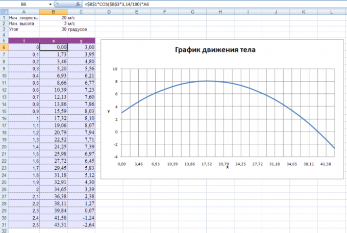
We can build a graph using the formula. To do this in the top cell of the second column enter the formula with the proviso that instead of the X variable will use the cell address of the first column and before the formula will be a =sign(e.g. =A1*A1 meets x*x). Then just drag this cell down as you did in the first paragraph.

To build the graph left to highlight both columns and to perform simple surgery. To do this open the "chart Wizard" icon located on the toolbar). Select a Scatter chart with curves (you can choose more scatter with markers, depending on your preference) and then click "OK" several times. The schedule is ready.