As in Excel to build a direct

Microsoft Office Excel has built-in tools based on tabular data to create charts of different types. A graph that can show a direct line here is also related to the diagrams. In Excel and the ability to fill the table with data, calculated according to the formulae given by the user, so the task of building a straight with the use of this program can be attributed to the discharge is not very complicated.

You will need

The table editor Microsoft Office Excel 2007 or 2010.

Instruction

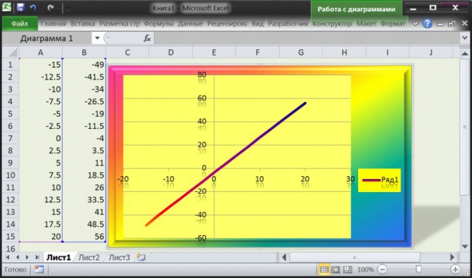
Launch Excel and complete the two columns created by default, the worksheet with an empty table. The first column should contain a list of points along the x-axis, which should be present on the chart with a straight line. Place in the top cell (A1) in this column the minimum value along the X-axis, for example, -15.

The second line of the column, type an equal sign, then click the mouse pointer to the previous cell, type a plus sign and type the number corresponding to the amount of the increment for each successive point on the x-axis. For example, to between points along the X-axis is the distance in 2.5 points, the contents of this cell (A2) should be: =A1+2,5. To finish entering the formula, press Enter.

Move the mouse pointer to the bottom right corner is filled in cells of a table, and when the pointer transformirovalsya in the black plus sign and drag the cell down to the last row of data column. For example, if you want to direct was built on 15 points, dragged the selection to the cell A15.

In the first row of the second column (B1) type the algorithm for calculating the points of a straight line. For example, if they must be calculated by the formula y=3x-4, the contents of the cell should be: =3*A1-4. After you press Enter and drag this cell to the full height of the table described in the previous step.

Select both filled column and then click the "Insert" menu in Excel. In the group of commands Charts open the drop-down list of "Point" and select the most suitable type of chart. Immediately after that, the table editor will calculate the point and place chart on the same sheet of paper.

Using the three tabs combined with the title "Working with diagrams", give the desired look created by the graphics. These tabs application adds in a menu after creating a new chart, and later you can call them with the line chart selected by mouse click.

Is the advice useful?