How to build a histogram in Excel

The histogram is a graph in which the data is displayed in columns. The height of the columns depends on amount of data, and the interval between them – from the period of time during which these data were collected.

Instruction

1. Create a table and enter data, based on which you will build the histogram.
   
   
2. Select random cell from the table. In the menu "Insert" select "Chart" or click on the icon "chart Wizard" on the toolbar. To create a histogram with the default settings, after selecting the cell, press F11. The histogram is created on a separate sheet.
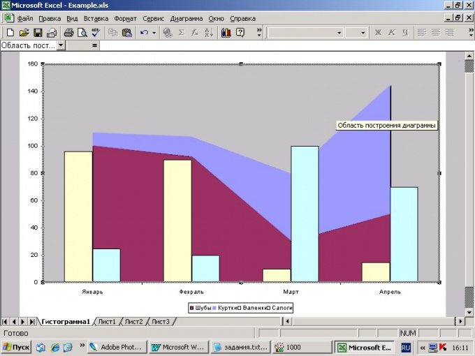
3. Select from the list the type "Histogram". In the "Appearance" section, specify the subtype. In the lower window is displayed in a tooltip-a description that will help you to make a choice. Click on the "Result" to see how it will look like the histogram based on your data. Go to the tab "Custom" if you want to create a custom histogram – for example, in combination with the chart, or area. To continue the build, click Next.
4. In the next window you should specify the range of data to build the histogram. The default is whole table. Highlight those cells whose content should be displayed in the histogram. In the "Range" dialog box, specify the desired values. With the switch from "Rows" to determine which setting will be indicated on the horizontal axis – the rows or columns. Click "Next" to continue.
5. In the "chart Options" on the tab "Headers" provide a title for your histogram and axes, if they deem it necessary. Navigating the tabs, you can make drawing in line with job he needs to illustrate. In the preview window displays all the changes you make. To continue, click "Next".
6. In the last step, specify the Excel editor, where you intend to place the histogram to embed it in a worksheet or placed on a separate sheet. Select the desired value and click "finish" to complete the work.