
Instruction
1
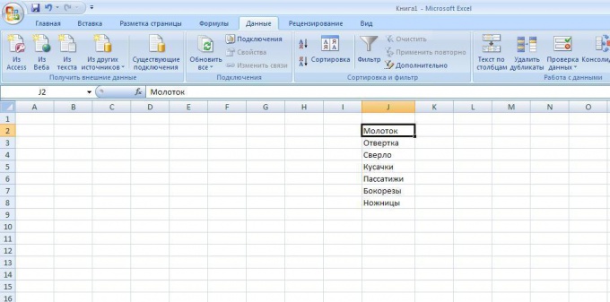
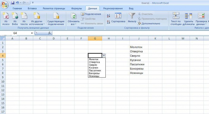
First you need to compile the list of interesting items. They should be placed in the order in which you want to appear.
2
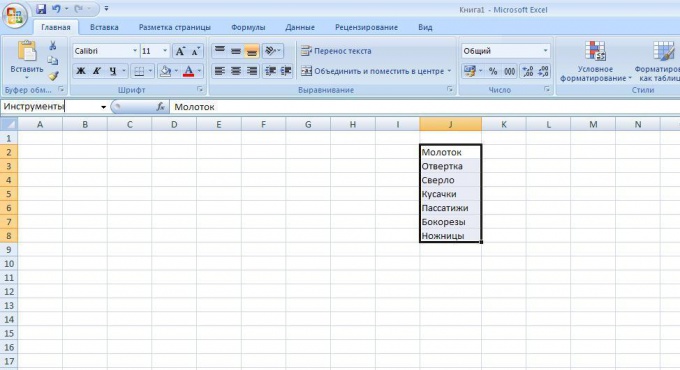
You now need to allocate the list and assign it a name. It should be administered in line in the upper left corner where usually is written the address of the cell. In our example the list is named "Tools".
3
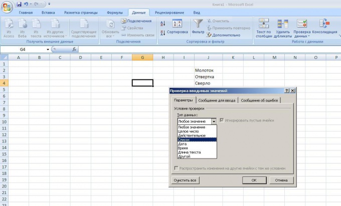
Next, select the cell in which you want to create a list, for example, it is G4. Then in the tab "Data" click "data Validation". In the opened window, in the field "data Type" choose "List".
4
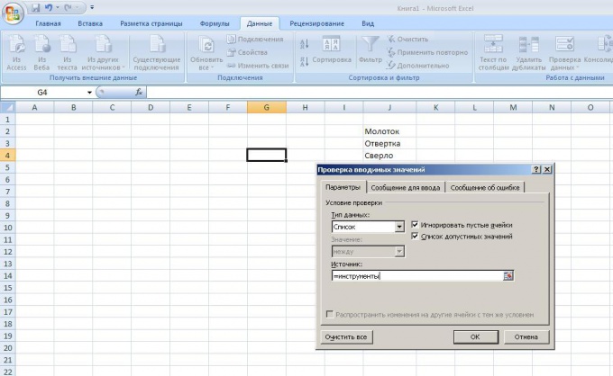
After that, the window should appear in the line "Source." It is necessary to specify the list name after the " = " sign, and click "OK".
5
Now in the specified cell, you can select an item from the list specified by us. If you want to make the same list in a different place, you can just copy and then paste it wherever you want, even on another sheet.
6
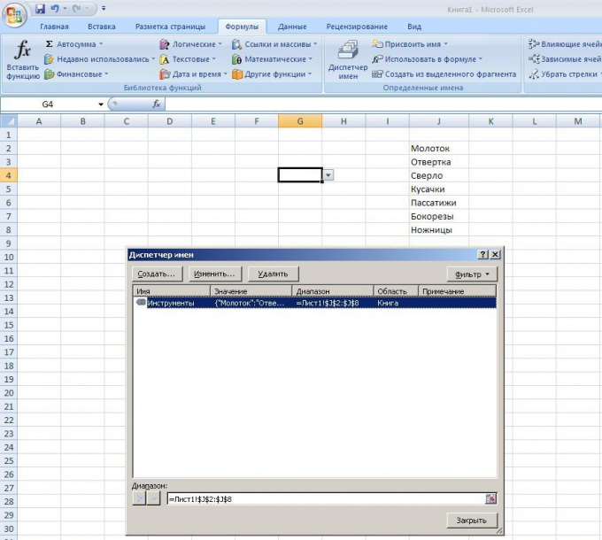
To view all the lists created in this file, you can click on "name Manager" in the tab "Formulas". Here you can create, delete and change your lists, and view their properties.
7
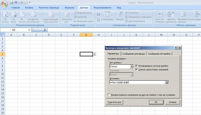
If there is a need to create a drop-down list on the adjacent sheet, select the cell, click "Data" then "data Validation". In the row "data Type" select "List" and the "Source" you need to specify the sheet name and range. The name of the list in this case will not fit. In our example, the list of items are located in the range at J2, J8, so I write =Sheet1!$J$2:$J$8. This range can be copied from the name Manager in the Formulas tab.
8
The easiest way to create drop down list in Excel is to press Alt + ↓. It is necessary to select the cell immediately adjacent list items. I.e. in the example described above, this technique will only with cells J1 and J9. Of course, the functionality of this method is very limited, but in certain cases it can be useful.