How to make a dropdown list in Excel

In Microsoft Excel is very easy to work with different tables for calculations. Based on them you can create reports, build charts of different types and graphics. When working with data one of the supporting elements in Excel is a drop-down list. With this element the user can select one value from a range of preset, the same type of data. Setting the drop-down list is in Excel. You can set the drop-down list through the appointment of a special type for the data range, or when using the control.

Instruction

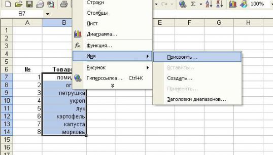
1. In a table or list, select the cells containing the data you want to put in a drop-down list. In the menu select "Insert" - "Name" "Assign". Further, in the requested field, type a name for the selected range and click "OK".
2. In the worksheet, select the cell to set the drop-down list. In the menu open "Data" - "Validation". After that navigate to new window in the tab "Settings" in the dialog field "data Type" insert the string "List". At the same time in the same window will appear the "Source". Enter the symbol "=" and the name of the selected range, which was specified cells with the data. To apply settings press "Enter" or "OK". This is the most simple variant of the drop-down list.
3. At the same time in the same window will appear the "Source". Enter the symbol "=" and the name of the selected range, which was specified cells with the data. To apply your selections, click "Enter" or "OK". This is the most simple variant of the drop-down list.
4. In Excel there is no way to set the drop-down list with a more complex design. To do this, use the control called "list box", inserted into the Excel worksheet. To install it, open the menu "View" then "toolbars" and "Forms".
5. Click on the opened panel controls icon combo box" - this is a drop-down list. Draw with the mouse a rectangle in the form fields. Highlight, right-click the drawn list, and specify the Format of the object...".
6. In the dialog box in the "create a list range set the desired range of cells. To do this, the mouse select the cells which should be in the drop-down menu of Excel. In the field "cell Link box, select the location number to output the sequence number of the item selected in the list. Specify the number of rows in a generated list. The "OK" button will apply all settings, and the list is ready to use.