
Instruction
1
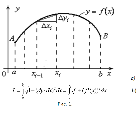
The first case (flat). Let IAV is set to a flat curve y = f(x). The argument of the function will change in the range from a to b and it is continuously differentiable this segment. Find the length L of the arc IAV (Fig. 1A). To solve this problem, break the reporting period into elementary segments ∆xi, i=1,2,...,n. As a result, the IAV will be divided into elementary arcs ∆Ui, plots the graph of y=f(x) at each of the elementary segments. Find the length ∆Li of an elementary arc approximately, replacing it with the corresponding chord. It is possible to increase in to replace the differentials and use the Pythagorean theorem. After the issuance of the square root of the differential dx will get the result shown in figure 1b.
2
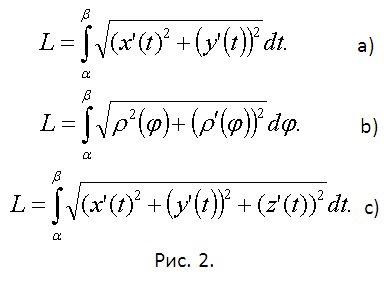
The second case (arc IAV set parametrically). x=x(t), y=y(t), tє[α,β]. Function x(t) and y(t) have continuous derivatives on the interval this interval. Find their differentials. dx=f’(t)dt, dy=f’(t)dt. Substitute these differentials into the formula to calculate the length of the arc in the first case. Remove dt from the square root under the integral, put x(α)=a, x(β)=b and come to the formula for calculating arc length in this case (see Fig. 2A).
3
The third event. Arc IAV graph of a function given in polar coordinates ρ=ρ(φ) of the Polar angle φ during the passage of the arc changes from α to β. The function ρ(φ)) has a continuous derivative on the interval of consideration. In such a situation, the easiest way to use the data obtained in the previous step. Choose φ as a parameter and substitute in equations relating polar and Cartesian coordinates x=ρcosφ y=ρsinφ. Differentiate the formula and substitute the squares of the derivatives in the expression in Fig. 2A. After a bit of identical transformations that are based mainly on the use of trigonometric identities (cos)^2+(sinφ)^2=1 we obtain the formula for arc length in polar coordinates (see Fig.2b).
4
The fourth case (spatial curve, defined parametrically). x=x(t), y=y(t), z=z(t), tє[α,β]. Strictly speaking, we should apply the line integral of the first kind (the arc length). Curvilinear integrals calculated by translating them in ordinary certain. As a result, the practical answer remains the same as case two, the only difference is that under the root will appear in an extension term – the square of the derivative z’(t) (see Fig. 2C).