Instruction
1
The essence of linear interpolation can be described by the following assumption: in the interval between the known neighbouring tabular values of the argument xi and xj consider the function y=f(x) can be approximately regarded as linear. In other words, in this range the value function is proportional to the change in the argument.
2
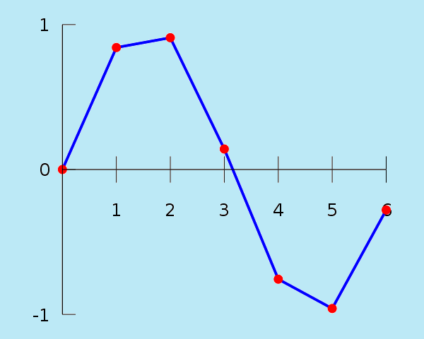
More clearly this assumption can be shown in graphic form in the Cartesian coordinate system. Consider the cut functions u and u appears to be a continuous straight line with known coordinates. When searching for intermediate values of the function Y, unknown argument X is between adjacent values XI and xj. Thus, we can write the following inequalities XI < X < xj, yi < Y < yj.
3
Express written terms of proportions of the following: (yj – yi)/(xj – XI) = (Y – yi)/(X – XI). Here yj and xj is the target value, yi, XI – initial value of the segment, X and Y – the desired intermediate values.
4
As can be seen from the proportions for a given increment of the argument X - XI it is easy to find the corresponding change of the function Y – yi. Express the increment: Y – yi = ((yj – yi)/(xj – XI))*(X – XI).
5
Thus, the intermediate function values can be determined, knowing only the increment on which there is a change of argument. Calculate the difference yj – yi xj – XI at a given step of the argument X – XI. Substituting these values in the formula increment, find the rate of change of a function.
6
Find the intermediate value Y. For this to the increment value add to the initial figure o functions on the considered segment. Likewise, is any intermediate value with a specified step increment.
7
If there is a problem in defining X for given values of the function y=f(x) is the inverse linear interpolation. Its essence is finding values of X using the same proportion, but now as a known parameter is the increment of the function Y – u. Using a similar transformation is unknown intermediate value of the argument X = ((yj – yi)/(xj – XI))/(Y – u) + XI.